Overview
The fundamental challenge of machine learning is to find a response function
{% f:X \mapsto Y %}
that minimizes risk, defined as
{% Risk = \mathbb{E}[ L(x,y, f(x)) ] %}
The challenge of machine learning is that typically the distribution of {% \mathbb{P}(x,y) %} is unknown.
Hypothesis Set
The process of training a machine learning algorithm is essentially the process of finding a function among a set of functions which minimizes the risk, defined above. That is, the analyst identifies a set of functions (for example, all linear functions) which is called the Hypothesis set, or Hypothesis space, {% H %}.
{% f \in H %}
Then the analyst attempts to identify the function (here labeled {% f^* %}) within that set which minimizes the risk.
{% f_H = arg \; min_{f \in H} \; \mathbb{E}[ L(x,y, f(x)) ] %}
When the Hypothesis set under consideration is the class of all functions ({% H_{all} %}), the resulting function {% f_H %} is referred to as the
Bayes classifier, and labeled {% f_{bayes} %}.
Because the distribution that generates the data is rarely known, the process of minimizing the risk typically involves minimizing the empirical risk, see below.
Empirical Loss Minimization
The empirical loss function is a measure of the loss on the given dataset. It is defined as
{% R_{emp} (f) = \frac{1}{n} \sum_{i=1}^n l(x_i,y_i,f(x_i)) %}
The empirical loss is generally taken to be a proxy for the loss given above, which leads one to try to find the
function that minimizes the empirical loss use that function as the trained model.
{% f_{emp} = arg \; min \; \mathbb{E}[ L(x,y, f(x)) ] %}
Empirical Loss Minimization on a Parametric Hypothesis Space
An example of empirical loss minimization is OLS Regression. In this case, the Hypothesis set is the set of linear functions
{% y = ax + b %}
The loss is defined to be the squared error
{% loss = \sum[y(x) - (ax_i +b)]^2 %}
Given a dataset, the procedure using analytic
optimization
techniques to find the values of {% a %} and {% b %} that minimize the squared loss.
Error Decomposition
The error of a given chosen function {% f_i %} is defined to be
{% R(f_i) - R(f_{bayes}) %}
That is, it shows the difference between the risk of the chosen function and the risk of the optimal
function (the Bayes classifier).
The error can be decomposed as the sum of two terms, the estimation error and the approximation error.
{% R(f_i) - R(f_{bayes}) = (R(f_i) - R(f_H)) + (R(f_H)-R(f_{bayes})) %}
Where
{% estimation \; error = (R(f_i) - R(f_H)) %}
{% approximation \; error = (R(f_H)-R(f_{bayes})) %}
Misfitting
- Underfitting
When the hypothesis set is chosen to be small, the result can be underfitting. That is, there is a large approximation error.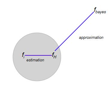
- Overfitting
When the hypothesis set is large, this can result in a large estimation error, even though the approximation error is small.The size of the Hypothesis set is often referred to as the model complexity. That is, complex models can implement a large set of functions.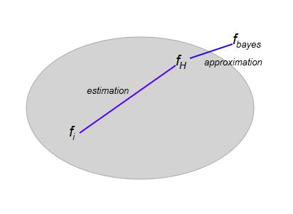
Bias Variance Tradeoff
Bias Variance Tradeoff mathematically shows the relationship of model error to model complexity.
Generalization
Generalization is the ability of a response function to be able to accurately predict response values to inputs that are not in the training set. In terms of risk, a function that generalizes is one that actually minimizes the risk, as opposed to memorizing the training set.
The sample function given above that memorizes the training set does not generalize well. The key to generalization is to constrain the set of response functions to a set that exludes the functions that dont generalize. For example, if the lookup function is not among the set of functions that available to choose as a response function, then it will not be chosen in the loss minimization procedure.
The above shows a hypothetical graph of the Generalization Error versus the number of response function degrees of freedom. At first, as the degrees of freedom is increased, the model reduces its generalization error, as it moves from being underfit to fit. Eventually, the model becomes overfit as additional parameters as added, and the generalization error starts to go up with each additional degree of freedom.
- out of sample error -
- in sample error - this is the measured error of the response function to the training data
- model complexity - is a measure of the model complexity, typically
Parametric Response Function
The standard way to constrain the set of available response functions is to choose a function that is dependent on a set of parameters as the template for the response function. That is, the set of available functions all have the same form, only differing in the value of a set of parameters.
As an example, the following function can serve as the response function template
{% f(x) = a + bx + cx^2 %}
where a,b,c are parameters.
Once the response function has been chosen to be a parametric function, an optimization procedure needs to be chosen that can find the parameters that minimizes the loss. There are generally two methods to achieve this.
- Gradient Descent is the standard tool used to find the function that minimizes the loss. However, the basic method of numerically computing the gradient of the response function for use within gradient descent can be computationally expensive.
- Backpropagation is designed to speed up the gradient descent procedure outlined above by using the chain rule to compute the gradient of the response function without having to rely the standard numeric method.